Handling processed AQG data
Once the raw data is processed and converted into an AQGDataset-class, all further visualization and offered methods are carried out on this variable.
General routine for processed AQG data
- processing of time series data has been finished
- final result (mean absolute gravity value) can be obtained
- additionally, several aspects of the data can be expored and visualized (see list below)
- the data is archived in a reproducible way (netCDF-file with metadata for reproducibility)
Which functionalities this AQGDataset-class offers
- retrieve processed gravity time series signal
- calculate final absolute mean value
- transfer gravity value to differen height
- calculate Allan Deviation
- compare AQG time series to reference data time series
- resample time series data
- archive data (as NetCDF)
- plot Allan Deviation
- plot full gravity signal
- calculate statistics (SEM, SD_h, TAV, sensitivity)
- generate measurement report as PDF
- plotting of all available variables (after manual extraction from class)
Read processed data from an .nc-file
read_aqg_dataset() uses xarray.open_dataset() to create an xarray.Dataset instance, and then wraps it as an AQGDataset.
from gravitools.aqg import read_aqg_dataset
dataset = read_aqg_dataset("../data/test.nc")
dataset
<AQGDataset: 20240620_163341>
Save to file
AQGDataset.to_nc() exports the dataset as NETCDF4, a binary data format. The resulting file contains the full signal of all data columns and all relevant metadata. It is also transparently compressed.
dataset.to_nc("../data/test.nc")
Accessing dataset properties and metadata
AQGDataset is a wrapper to an xarray.Dataset, which provides advantages for reading the data from file since individual columns can be read on-demand. The AQGDataset.ds attribute can also be accessed directly, though this is usually not needed. All metadata is contained in the ds dataset and can be accessed via AQGDataset.ds.attrs, which is also accessible with the AQGDataset.metadata property.
dataset.ds.attrs["software"]
'1.7.4'
dataset.metadata["software"]
'1.7.4'
List of properties
For all available class-properties please see the corresponding api documentation.
The can be assesd via dataset.<property_name>.
Accessing dataset variables
For individual visualization, extraction or processing, all available time series signal can be extracted from the xarray.Dataset.
A list of available variables can be shown.
dataset.ds.data_vars
Data variables:
    gps_timestamp                      (utc) float64 391kB ...
    gps_state                          (utc) int64 391kB ...
    ref_time_mode                      (utc) object 391kB 'S' 'S' ... 'S' 'S'
    g_raw                              (utc) int64 391kB ...
    dg_tilt                            (utc) float64 391kB ...
    dg_pressure                        (utc) float64 391kB ...
    dg_earth_tide                      (utc) int64 391kB ...
    dg_polar                           (utc) float64 391kB ...
    atmospheric_pressure               (utc) float64 391kB ...
    external_temperature               (utc) float64 391kB ...
    sensor_head_temperature            (utc) float64 391kB ...
    vacuum_chamber_temperature         (utc) float64 391kB ...
    tiltmeter_temperature              (utc) float64 391kB ...
    x_tilt                             (utc) float64 391kB ...
    y_tilt                             (utc) float64 391kB ...
    sat_abs_offset_correction          (utc) int64 391kB ...
    sat_abs_offset_correction_applied  (utc) int64 391kB ...
    raw_quartz_frequency               (utc) float64 391kB ...
    cooler_phi                         (utc) float64 391kB ...
    cooler_eta                         (utc) float64 391kB ...
    rep_phi                            (utc) float64 391kB ...
    rep_eta                            (utc) float64 391kB ...
    atoms_number                       (utc) int64 391kB ...
    laser_temperature                  (utc) float64 391kB ...
    is_outlier                         (utc) bool 49kB ...
    g                                  (utc) float64 391kB ...
dataset.get("g_raw")
utc
2024-06-20 16:33:41.790999889    9808372019
2024-06-20 16:33:42.332000017    9808372002
2024-06-20 16:33:42.871999979    9808372150
2024-06-20 16:33:43.411000013    9808372094
2024-06-20 16:33:43.950999975    9808372088
                                    ...
2024-06-20 23:59:57.690000057    9808372158
2024-06-20 23:59:58.230000019    9808372119
2024-06-20 23:59:58.769999981    9808372203
2024-06-20 23:59:59.309999943    9808372333
2024-06-20 23:59:59.848999977    9808372214
Name: g_raw, Length: 48859, dtype: int64
Viewing the gravity time series
Usually it is not necessary or meaningfull to consider individual drops because the variance is very high and, due to the nature of the measurement principle, successive drops are correlated. For this reason, AQGDataset provides two methods for accessing the gravity signal:
AQGDataset.full_g(): The full gravity signal, showing all drops at 0.54 s intervals. Note that this does not follow a white noise distribution.
AQGDataset.g(): The gravity signal downsampled to 10 second interval means. If there are no interruptions to the measurement, a 10 second interval contains 18 or 19 drops. Importantly, one this time scale, the signal does show a white noise distribution.
# Configure Pandas display float precision
import pandas as pd
pd.options.display.float_format = '{:.1f}'.format
dataset.full_g()
GravityTimeSeries: 20240620_163341
{'vgg': Gradient(value=-3287.0, error=0), 'height': 0.0}
                                         y
utc
2024-06-20 16:33:41.790999889 9808373525.6
2024-06-20 16:33:42.332000017 9808373508.7
2024-06-20 16:33:42.871999979 9808373656.6
2024-06-20 16:33:43.411000013 9808373600.7
2024-06-20 16:33:43.950999975 9808373594.7
...                                    ...
2024-06-20 23:59:57.690000057 9808373558.5
2024-06-20 23:59:58.230000019 9808373519.9
2024-06-20 23:59:58.769999981 9808373603.8
2024-06-20 23:59:59.309999943 9808373733.8
2024-06-20 23:59:59.848999977 9808373615.2

[48690 rows x 1 columns]
dataset.g()
GravityTimeSeries: 20240620_163341
{'vgg': Gradient(value=-3287.0, error=0), 'height': 0.0}
                               y  y_err  y_count
utc
2024-06-20 16:33:40          NaN   22.9        6
2024-06-20 16:33:50 9808373396.7   40.9       19
2024-06-20 16:34:00 9808373739.8   25.0       18
2024-06-20 16:34:10 9808373609.3   52.7       19
2024-06-20 16:34:20 9808373557.8   70.4       19
...                          ...    ...      ...
2024-06-20 23:59:20 9808373165.9   16.3       19
2024-06-20 23:59:30 9808373276.3   28.3       18
2024-06-20 23:59:40 9808373422.4   37.6       19
2024-06-20 23:59:50 9808373267.2   46.0       19
2024-06-21 00:00:00          NaN   86.3        9

[2679 rows x 3 columns]
You can obtain the gravity signal at a different transfer height by transferring this result (dataset.g().transfer(h=0)) or by providing a height argument (dataset.g(h=0)).
When further downsampling to 10 minute intervals, for instance, the errors (standard error of the mean) should accurately represent the statistical uncertainty.
dataset.g().resample("10min")
GravityTimeSeries: 20240620_163341
{'vgg': Gradient(value=-3287.0, error=0), 'height': 0.0}
                               y  y_err  y_count
utc
2024-06-20 16:30:00 9808373506.7   51.7        7
2024-06-20 16:40:00 9808373455.7   19.5       56
2024-06-20 16:50:00 9808373425.0   22.0       60
2024-06-20 17:00:00 9808373455.7   16.7       60
2024-06-20 17:10:00 9808373465.0   18.3       60
2024-06-20 17:20:00 9808373487.8   17.2       50
2024-06-20 17:30:00 9808373446.3   21.9       60
2024-06-20 17:40:00 9808373438.4   17.1       60
2024-06-20 17:50:00 9808373438.0   14.9       60
2024-06-20 18:00:00 9808373412.2   17.6       60
2024-06-20 18:10:00 9808373418.2   18.3       60
2024-06-20 18:20:00 9808373394.1   19.7       60
2024-06-20 18:30:00 9808373425.3   18.8       60
2024-06-20 18:40:00 9808373485.1   18.7       60
2024-06-20 18:50:00 9808373387.6   16.0       55
2024-06-20 19:00:00 9808373469.7   16.4       60
2024-06-20 19:10:00 9808373406.8   19.3       60
2024-06-20 19:20:00 9808373401.9   17.1       60
2024-06-20 19:30:00 9808373418.5   18.9       60
2024-06-20 19:40:00 9808373448.6   17.4       58
2024-06-20 19:50:00 9808373493.5   17.8       60
2024-06-20 20:00:00 9808373480.7   14.1       60
2024-06-20 20:10:00 9808373462.0   15.6       60
2024-06-20 20:20:00 9808373426.4   17.8       50
2024-06-20 20:30:00 9808373440.2   16.7       60
2024-06-20 20:40:00 9808373514.6   17.7       60
2024-06-20 20:50:00 9808373492.9   18.6       60
2024-06-20 21:00:00 9808373437.1   17.5       58
2024-06-20 21:10:00 9808373420.2   19.0       60
2024-06-20 21:20:00 9808373413.2   18.4       60
2024-06-20 21:30:00 9808373426.9   23.2       60
2024-06-20 21:40:00 9808373435.2   17.2       60
2024-06-20 21:50:00 9808373427.7   16.6       55
2024-06-20 22:00:00 9808373456.1   18.0       60
2024-06-20 22:10:00 9808373422.9   20.9       60
2024-06-20 22:20:00 9808373424.0   18.3       60
2024-06-20 22:30:00 9808373453.9   19.0       60
2024-06-20 22:40:00 9808373486.4   18.2       60
2024-06-20 22:50:00 9808373473.6   15.1       60
2024-06-20 23:00:00 9808373433.7   16.9       60
2024-06-20 23:10:00 9808373433.4   19.1       60
2024-06-20 23:20:00 9808373484.8   18.7       50
2024-06-20 23:30:00 9808373485.6   17.6       60
2024-06-20 23:40:00 9808373393.7   16.1       60
2024-06-20 23:50:00 9808373384.0   17.9       60
2024-06-21 00:00:00 9808373349.8   26.0       30
Naturally, some intervals will not contain as many drops and the statistical error can therefore be much higher. You can exclude these intervals by requiring at least 50% of the max. number of drops within an interval, for instance.
interval = "10min"
g = dataset.g().resample(interval, min_count=0.5)
g
GravityTimeSeries: 20240620_163341
{'vgg': Gradient(value=-3287.0, error=0), 'height': 0.0}
                               y  y_err  y_count
utc
2024-06-20 16:30:00          NaN   51.7        7
2024-06-20 16:40:00 9808373455.7   19.5       56
2024-06-20 16:50:00 9808373425.0   22.0       60
2024-06-20 17:00:00 9808373455.7   16.7       60
2024-06-20 17:10:00 9808373465.0   18.3       60
2024-06-20 17:20:00 9808373487.8   17.2       50
2024-06-20 17:30:00 9808373446.3   21.9       60
2024-06-20 17:40:00 9808373438.4   17.1       60
2024-06-20 17:50:00 9808373438.0   14.9       60
2024-06-20 18:00:00 9808373412.2   17.6       60
2024-06-20 18:10:00 9808373418.2   18.3       60
2024-06-20 18:20:00 9808373394.1   19.7       60
2024-06-20 18:30:00 9808373425.3   18.8       60
2024-06-20 18:40:00 9808373485.1   18.7       60
2024-06-20 18:50:00 9808373387.6   16.0       55
2024-06-20 19:00:00 9808373469.7   16.4       60
2024-06-20 19:10:00 9808373406.8   19.3       60
2024-06-20 19:20:00 9808373401.9   17.1       60
2024-06-20 19:30:00 9808373418.5   18.9       60
2024-06-20 19:40:00 9808373448.6   17.4       58
2024-06-20 19:50:00 9808373493.5   17.8       60
2024-06-20 20:00:00 9808373480.7   14.1       60
2024-06-20 20:10:00 9808373462.0   15.6       60
2024-06-20 20:20:00 9808373426.4   17.8       50
2024-06-20 20:30:00 9808373440.2   16.7       60
2024-06-20 20:40:00 9808373514.6   17.7       60
2024-06-20 20:50:00 9808373492.9   18.6       60
2024-06-20 21:00:00 9808373437.1   17.5       58
2024-06-20 21:10:00 9808373420.2   19.0       60
2024-06-20 21:20:00 9808373413.2   18.4       60
2024-06-20 21:30:00 9808373426.9   23.2       60
2024-06-20 21:40:00 9808373435.2   17.2       60
2024-06-20 21:50:00 9808373427.7   16.6       55
2024-06-20 22:00:00 9808373456.1   18.0       60
2024-06-20 22:10:00 9808373422.9   20.9       60
2024-06-20 22:20:00 9808373424.0   18.3       60
2024-06-20 22:30:00 9808373453.9   19.0       60
2024-06-20 22:40:00 9808373486.4   18.2       60
2024-06-20 22:50:00 9808373473.6   15.1       60
2024-06-20 23:00:00 9808373433.7   16.9       60
2024-06-20 23:10:00 9808373433.4   19.1       60
2024-06-20 23:20:00 9808373484.8   18.7       50
2024-06-20 23:30:00 9808373485.6   17.6       60
2024-06-20 23:40:00 9808373393.7   16.1       60
2024-06-20 23:50:00 9808373384.0   17.9       60
2024-06-21 00:00:00 9808373349.8   26.0       30
Obtain mean gravity value
Calculate the dataset's mean gravity value (with a statistical error) at the standard transfer height (gravitools.utils.STANDARD_HEIGHT).
g_mean = dataset.mean()
g_mean
AbsGValue(value=np.float64(9808373441.901157), error=np.float64(19.447983338980816), height=0.0, vgg=Gradient(value=-3287.0, error=0))
str(g_mean)
'9,808,373,441.9 ± 19.4 nm/s² (0.0 m)'
The mean gravity at a different height can be obtained by transferring this value or by supplying a custom height to the mean() method.
str(g_mean.transfer(height=0))
'9,808,373,441.9 ± 19.4 nm/s² (0 m)'
str(dataset.mean(h=0))
'9,808,373,441.9 ± 19.4 nm/s² (0 m)'
Calculating statistics of the measurement
Calculate interesting standard statistics, which are also included in the measurement report.
dataset.get_statistics()
(np.float64(2.7663289116715513),
 np.float64(19.447983338980816),
 16.58154602293323,
 np.float64(479.71594261068253))
Visualizing the data
Set optional Matplotlib styling parameters
import matplotlib.pyplot as plt

plt.rcParams["figure.figsize"] = 8, 4
plt.rcParams["date.autoformatter.hour"] = "%H:%M\n%d %b"
plt.rcParams["axes.ymargin"] = 0.2
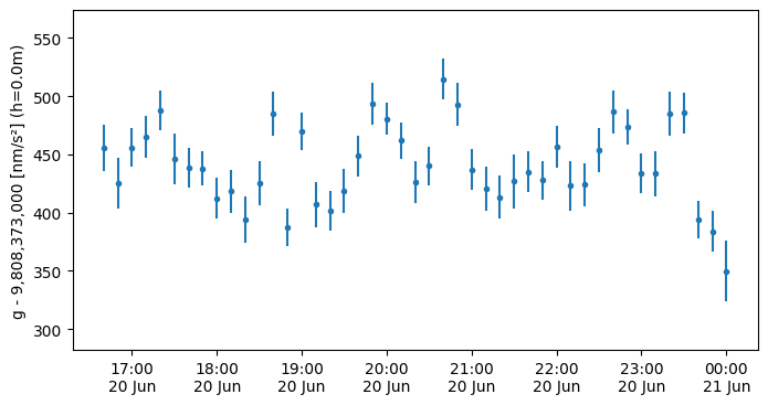
The GravityTimeSeries class provides a plot() method, which uses pyplot.errorbar() to create the graph.
g.plot()
<ErrorbarContainer object of 3 artists>
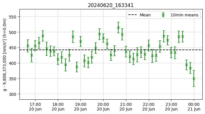
You can add more elements to the plot and customize it, just like any other matplotlib plot.
plt.figure()
g.plot("x", color="green", label=f"{interval} means", capsize=3)
plt.axhline(float(g_mean) - g.y0, label="Mean", color="k", linestyle="--")
plt.grid(color="lightgrey")
plt.title(dataset.name)
plt.legend(ncols=2)
plt.show()
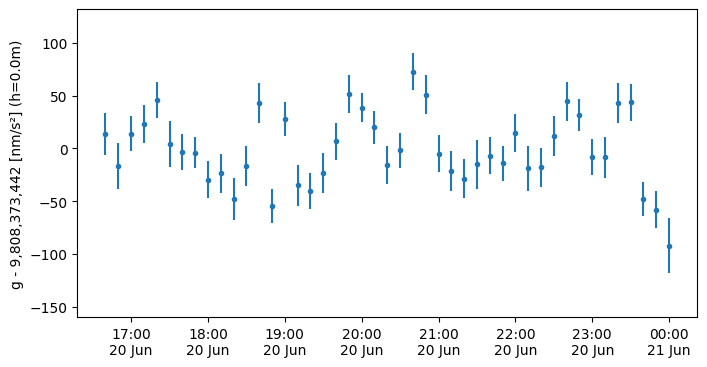
Plot the gravity signal relative to the mean gravity
g.plot(y0=float(g_mean))
plt.show()
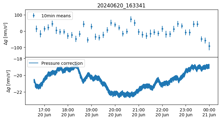
Create a stacked plot of the gravity signal and another data column
fig, axs = plt.subplots(nrows=2, sharex=True)
fig.subplots_adjust(hspace=0)
axs[0].set_title(dataset.name)
g.plot(ax=axs[0], y0=float(g_mean), label=f"{interval} means")
axs[1].plot(dataset.get("dg_pressure"), label="Pressure correction")
for ax in axs:
    ax.set_ylabel(r"$\Delta g$ [nm/s²]")
    ax.legend(loc="upper left")
plt.show()
Create plots of all available time series
Below is a generic method how all provided time series data can be easily plotted. The list of available variables can be shown as explained above. Here a relevant subset of this list (names can be used to replace the below example):
- g
- g_raw
- dg_earth_tide
- dg_tilt
- dg_pressure
- dg_polar
- atoms_number
# obtain data
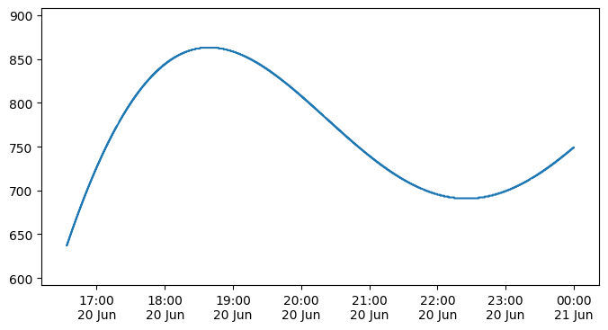
timeseries_parameter = dataset.get("dg_earth_tide")
# plot data
plt.plot(timeseries_parameter)
[<matplotlib.lines.Line2D at 0x7f494ee857f0>]
Create a standardized measurement report as PDF file
The AQGDataset-class provides the functionality to generate a standardized PDF report of the measurements.
This report intents to include all relevant information as well as standard plots of many important parameters.
dataset.save_report("../data/AQG_measurementReport.pdf")
<Figure size 1360x600 with 0 Axes>


<Figure size 1360x600 with 0 Axes>